Discovering slow modes from time-series data

In quantum mechanics, we have all information about how a system evolves if we know the evolution of each of its “independent orthogonal components” (aka “eigenstates”). This is also true for general dynamic systems: if we find such components (we call “slow modes”) and figure out their evolution, we get all information about its kinetics.

How do we find these slow modes? We use a similar idea to variational method in quantum mechanics. Basically we search in a function space for the slow modes (which are functions) with specific objectives and constraints. But unlike variational methods in QM, where we find eigenstates given the expression of the dynamic operator (Hamiltonian) but no observations, here we are interested in finding slow modes given time-series observations but no expression for the dynamic operator.

Let’s consider the 1st component: the slowest mode of the system. We want to find the function in a function space that is slowest (formally, meaning that the function f(x) has maximum autocorrelation given the time series data). How do we define a function space? A simple way is to first define a few basis functions and define the function space to be all possible linear combinations of these basis functions.

But would it affect our results if we do not have a good pre-defined basis functions? Yes, for instance if we use linear functions as basis functions (known as TICA), then it is not possible to capture nonlinear slow modes, which could be a big issue as many systems are intrinsically nonlinear.

Is it possible to adapt basis functions to data? Yes, one way is to use kernel methods where we do not explicitly specify basis functions, but instead specify the similarity measure among data and basis functions are determined accordingly. The problem is, the similarity measure is universal, which controls the “resolution” of the learned function. If a slow mode has super fine details in some parts while do not have many details in others, we may want to have different “resolutions” in different regions to be efficient, which cannot be done with kernel methods.

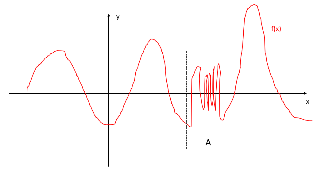
Consider following example, suppose f(x) is the slowest mode, which has a crazily oscillating part A together with smooth regions outside A:

If we use a low “resolution”, we do not need many data points to learn it, for instance we pick following data points (smiling faces):

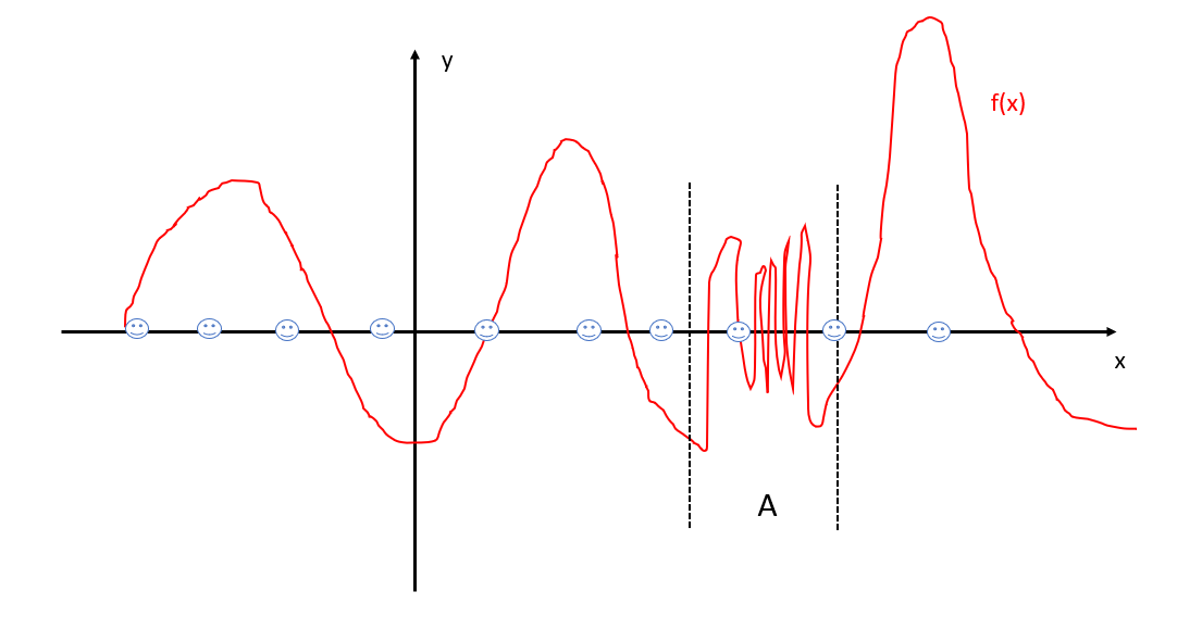
We are almost for sure that we lose all details of region A. Can we add more points in A? That is not going to help, since the “resolution” is so low that all points in A seem roughly the same.

What if we use a much higher “resolution”? Now we need much more data, like this:

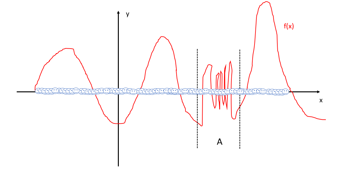
It is fine and should resolve all details, but here comes another issue: computation is too expensive. Since kernel methods require computing pairwise distance matrix which takes O(N^2) memory (N is number of points used). Moreover, computation involves solving generalized eigenvalue problem, which takes O(N^3) time. This means we cannot feed this method with too many data points, which limits its ability for complex systems.

Can we have basis functions adapted to data with flexible “resolutions”? This is where neural networks come in. Due to universal approximation theorem, neural networks are flexible enough to approximate any continuous functions. Based on work of VAMPnets, we use neural networks to learn basis functions and simultaneously find the optimal linear combination to fit the slowest mode using data. We find this method is more accurate in discovering slowest mode. Moreover, it is much faster and much more memory efficient since this neural network based method only takes O(N) memory and O(N) time.

If you are interested in how to discover higher-order slow modes, and theoretical connection with transfer operator theory and other details, please checkout this paper. For implementation and application, checkout this GitHub repository.